Research Question

This task-based tutorial builds upon three previous tool-oriented tutorials build_bedpe, query_bedpe, and plot_contacts and also introduces an alternate solution using get_loops. Becoming familiar with these tools is recommended before diving into this tutorial. In this tutorial, we will explore two different approaches to answer the following questions:

For the SOX8 gene, which TSS-CpG pairings show the strongest and weakest acetylation signal in 3D space?

To answer this question, we will determine acetylation levels by assessing and visualizing the changes in H3K27ac HiChIP reads between DMSO (control) and dCBP1 (treatment) in the RH4 cell type. We will use bedtools to obtain the SOX8 TSS, the TAD in which SOX8 resides, as well as all the CpG sites within the TAD. Next, we will use build_bedpe to construct pairings between the SOX8 TSS and all CpG sites within the TAD, and determine contact frequencies of the pairings using query_bedpe. We will use plot_contacts to visualize the process and conclude with visualizations of both the strongest and weakest acetylation signals in our case vs control analysis.

To list all available data on the Tinker box, simply type the following command into the terminal window:

list_samples.sh

Let’s assign simple names to our control, treatment, and reference files:

control=RH4_DMSO
treatment=RH4_HDACi

TSS=~/lab-data/hg38/reference/gencode.TSS.200bp.hg38.bed
TAD=~/lab-data/hg38/reference/TAD_goldstandard_lift.hg38.bed
CPG=~/lab-data/hg38/reference/cpg.hg38.bed

Obtain TSS

Now that we have a TSS file ready, we can obtain the SOX8 TSS

cat $TSS | grep SOX8 > SOX8_tss.bed

Obtain TAD

Using the SOX8 TSS, we can fetch the TAD it resides in

bedtools intersect \
   -a SOX8_tss.bed
   -b $TAD \
   -wa -wb
   | cut -f 6-8 > SOX8_tad.bed

cat SOX8_tad.bed

chr16  790000  1259999

Obtain CpG sites

We now have the SOX8 TSS and the TAD it resides in. Using the SOX8 TAD, let’s now obtain all the CpG sites housed in it.

bedtools intersect \
   -a $CPG
   -b SOX8_tad.bed > SOX8_cpgs.bed

Visualize SOX8 TAD

We can now visualize the SOX8 TAD using plot_contacts. CpG sites and TSSs will be displayed by default.

plot_contacts.sh \
   --sample1 $control \
   --range chr16:790000:1260000:SOX8_TAD\
   --genome hg38 \
   --output_name SOX8.pdf \
   --norm aqua
   --max_cap 2 \
   --resolution 5000
   --annotations_default TRUE \
   --annotations_custom SOX8_tad.bed \
   --annotations_custom_color 657c78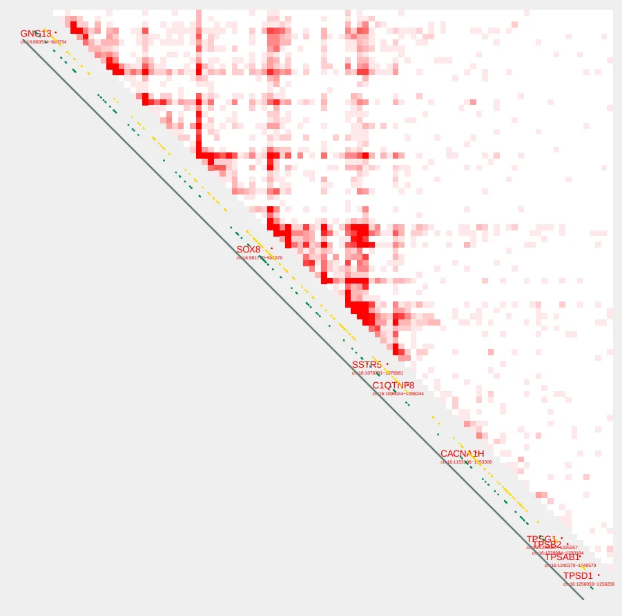

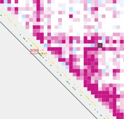
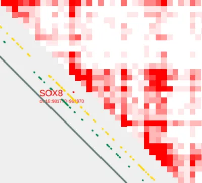
Let’s zoom in to SOX8.

Construct Pairs

Next, we can construct pairings between the SOX8 TSS and all CpG sites within the TAD by using build_bedpe.

build_bedpe.sh \
  -A SOX8_tss.bed \
  -B SOX8_cpgs.bed > SOX8_tss_cpg.bedpe

bedpe=SOX8_tss_cpg.bedpe

Visualize pairs

We can visualize these pairings using the --bedpe option with plot_contacts

plot_contacts.sh \
  -sample1 $control \
  -range chr16:790000:1260000:SOX8_TAD \
  -genome hg38 \
  -output_name SOX8_bedpe.pdf \
  -norm aqua \
  -resolution 5000 \
  -max_cap 2 \
  -bedpe $bedpe \
  -bedpe_color 424242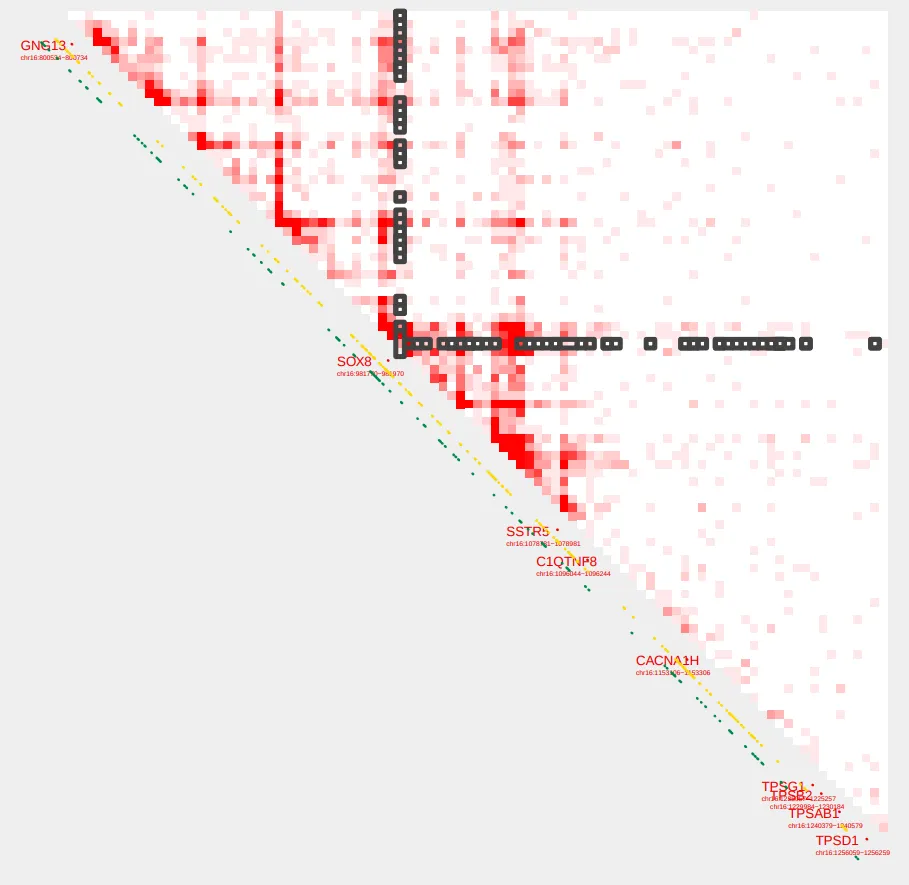

Obtain and sort contact frequencies

Great! We now have all the genomic pairings we want! We can now obtain the contact frequencies of these pairings using query_bedpe and sort them in increasing order

query_bedpe.sh \
   --sample1 $control \
   --sample2 $treatment \
   --pair SOX8_tss_cpg.bedpe \
   --genome hg38 --norm aqua --resolution 5000 \
   | sort -k9n > SOX8_tss_cpg_contact_values.bedpe

We can view the top and bottom values using head and tail commands. Since we sorted our list in increasing order, head will show us the smallest acetylation values and tail will show us the largest acetylation values.

head -n 5 SOX8_tss_cpg_contact_values.bedpe

chr16   979878   985327   chr16   981770	   981970   0.745   0      -0.745
chr16   807341   808025   chr16   981770	   981970   1.117   0.379  -0.738
chr16   817032   817833   chr16   981770	   981970   0.559   0      -0.559
chr16   869858   870117   chr16   981770	   981970   0.559   0      -0.559
chr16   800227   800806   chr16   981770	   981970   0.372   0      -0.372

tail -n 5 SOX8_tss_cpg_contact_values.bedpe

chr16   981770   981970   chr16   1089732   1089937   0       0.758   0.758
chr16   981770   981970   chr16    986820    987448   2.607   3.411   0.804
chr16   970219   971303   chr16    981770    981970   0.931   1.895   0.964
chr16   981770   981970   chr16   1050626   1050848   1.489   2.653   1.164
chr16   981770   981970   chr16   1057607   1057865   0       1.895   1.895

Visualize case-control pairs

Before we visualize the lowest and highest acetylation pairs, let’s visualize all of our pairs again, but this time we’ll look at both control and treatment samples using the two-sample version of plot_contacts

plot_contacts.sh \
   --sample1 $control \
   --sample2 $treatment \
   --range chr16:790000:1260000:SOX8_TAD \
   --resolution 5000 \
   --genome hg38 \
   --output_name SOX8_delta_all.pdf \
   --norm aqua \
   --max_cap 2 \
   --annotations_default TRUE \
   --annotations_custom SOX8_tad.bed \
   --annotations_custom_color 657c78 \
   --bedpe SOX8_tss_cpg.bedpe \
   --bedpe_color 424242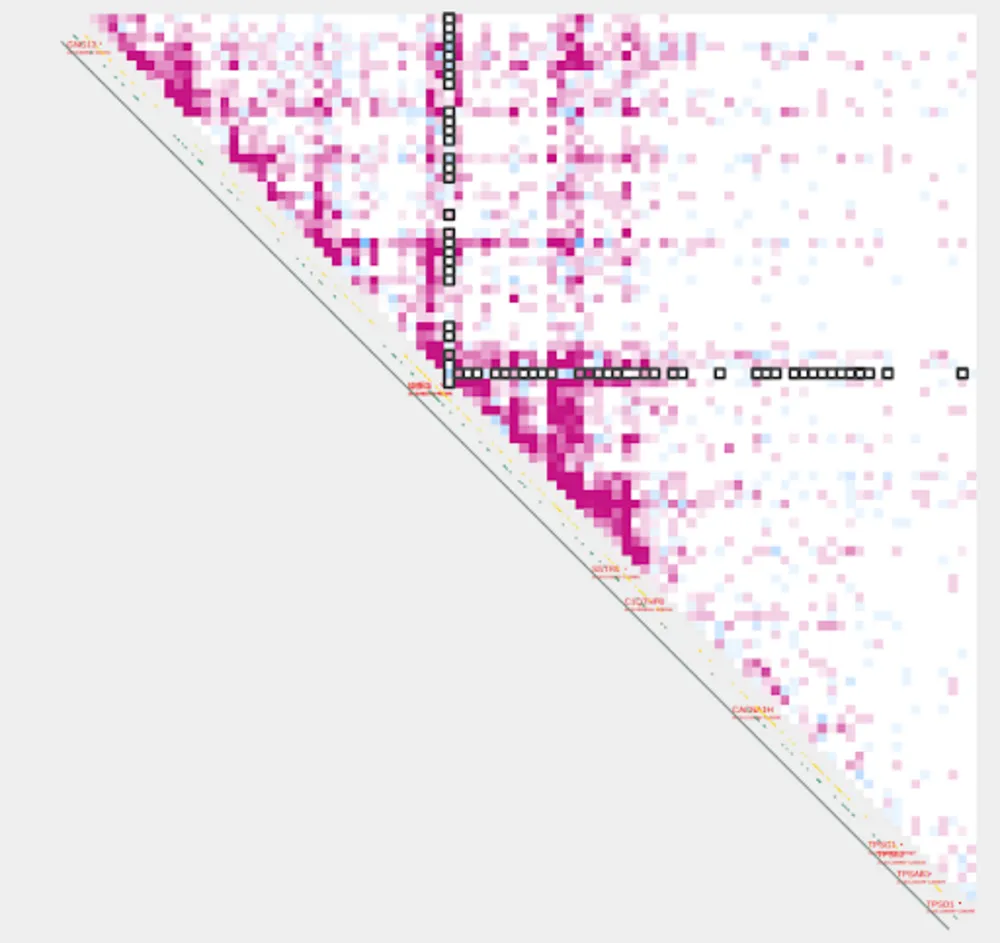

Save pairs with lowest and highest acetylation

Let’s save the pair with the lowest acetylation:

head -n 1 \
SOX8_tss_cpg_contact_values.bedpe > low_SOX8_tss_cpg_contact_values.bedpe

And let’s also save the pair with the highest acetylation:

tail -n 1 \
SOX8_tss_cpg_contact_values.bedpe > high_SOX8_tss_cpg_contact_values.bedpe

Visualize lowest and highest acetylation pairs

Now we can plug these bedpe files into the --bedpe option of plot_contacts to visualize the pairs with the lowest and highest acetylation values in our case vs control analysis.

plot_contacts.sh \
  --sample1 $control \
  --sample2 $treatment \
  --range chr16:790000:1260000:SOX8_TAD \
  --resolution 5000 \
  --genome hg38 \
  --output_name SOX8_delta_low.pdf \
  --norm aqua \
  --max_cap 2 \
  --annotations_default TRUE \
  --annotations_custom SOX8_tad.bed \
  --annotations_custom_color 657c78 \
  --bedpe low_SOX8_tss_cpg_contact_values.bedpe \
  --bedpe_color 424242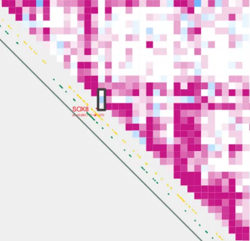

plot_contacts.sh \
  --sample1 $control \
  --sample2 $treatment \
  --range chr16:790000:1260000:SOX8_TAD \
  --resolution 5000 \
  --genome hg38 \
  --output_name SOX8_delta_high.pdf \
  --norm aqua \
  --max_cap 2 \
  --annotations_default TRUE \
  --annotations_custom SOX8_tad.bed \
  --annotations_custom_color 657c78 \
  --bedpe high_SOX8_tss_cpg_contact_values.bedpe \
  --bedpe_color 424242